Why can we have a Fast Fourier Transform ?
12 March 2009 at 3:23 pm 3 comments
The Fourier transform was introduced by Fourier as a tool to solve heat equations, but is now used in its discrete version throughout the computing world more than trillions of times each second. It is probably more, I was assuming an average computer does billions of Discrete Cosine Transforms per day for Web browsing (JPEG images and Youtube) and music listening, but how huge is the contribution of millions of people watching MPEG-2 compressed television programs on satellite or terrestrial digital broadcasting?
It is thus important to know that the Fourier transform (which is always the Fast Fourier Transform) is really fast (especially when it is dozens, hundreds of times faster than the natural algorithm). I am not yet sure about the fast versions of variants of the discrete transform (cosine transforms and its friends), but I guess they can be derived from the classical case.
What is it ?
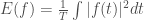
The classical Fourier transform takes a T-periodic function f and computes for each integer n the integral

where 


The discrete Fourier transform takes a discrete function given by 

which can also be represented by a matrix

where 

Other interpretations
The matrix 


Another way of saying the same thing is that the Fourier transform diagonalises product of polynomials (which corresponds to the convolution product of signals): the convolution product of two vectors is not easy to compute rapidly, but 


Keyword: tensor product
Humans would traditionally compute a Discrete Fourier Transform using the above formulas: each coefficient requires computing n products by roots of unity, giving the whole thing a complexity of n² operations. A little agebra will tell us how to give it a complexity of nk operations, when 
The key observation is that the matrix 


![A[(a_1, \dots, a_k), (b_1, \dots, b_k)] = A_1[a_1,b_1] \times](https://s0.wp.com/latex.php?latex=A%5B%28a_1%2C+%5Cdots%2C+a_k%29%2C+%28b_1%2C+%5Cdots%2C+b_k%29%5D+%3D+A_1%5Ba_1%2Cb_1%5D+%5Ctimes&bg=ffffff&fg=414141&s=0&c=20201002)
![A_2[a_1,b_2] \times \cdots \times A_k[a_k,b_k]](https://s0.wp.com/latex.php?latex=A_2%5Ba_1%2Cb_2%5D+%5Ctimes+%5Ccdots+%5Ctimes+A_k%5Ba_k%2Cb_k%5D&bg=ffffff&fg=414141&s=0&c=20201002)
For those of you who thrive on algebraic geometry and schemes, this translates into the following property: first remark that 


![Z_q = \mathrm{Spec}\ \mathbb C[X]/((X-1)(X-\zeta_q))](https://s0.wp.com/latex.php?latex=Z_q+%3D+%5Cmathrm%7BSpec%7D%5C+%5Cmathbb+C%5BX%5D%2F%28%28X-1%29%28X-%5Czeta_q%29%29&bg=ffffff&fg=414141&s=0&c=20201002)

![\frac{\mathbb C[X]}{(X^n-1)} \to \frac{\mathbb C[X_{k-1}]}{(X_{k-1}^2-1)} \otimes \frac{\mathbb C[X_{k-2}]}{(X_{k-2}-1)(X_{k-2}-i)} \otimes \frac{\mathbb C[X_{k-3}]}{(X_{k-3}-1)(X_{k-3}-\zeta_{k-3})}](https://s0.wp.com/latex.php?latex=%5Cfrac%7B%5Cmathbb+C%5BX%5D%7D%7B%28X%5En-1%29%7D+%5Cto+%5Cfrac%7B%5Cmathbb+C%5BX_%7Bk-1%7D%5D%7D%7B%28X_%7Bk-1%7D%5E2-1%29%7D+%5Cotimes+%5Cfrac%7B%5Cmathbb+C%5BX_%7Bk-2%7D%5D%7D%7B%28X_%7Bk-2%7D-1%29%28X_%7Bk-2%7D-i%29%7D+%5Cotimes+%5Cfrac%7B%5Cmathbb+C%5BX_%7Bk-3%7D%5D%7D%7B%28X_%7Bk-3%7D-1%29%28X_%7Bk-3%7D-%5Czeta_%7Bk-3%7D%29%7D&bg=ffffff&fg=414141&s=0&c=20201002)
![\otimes \cdots \otimes \frac{\mathbb C[X_0]}{(X_0-1)(X_0-\zeta)}](https://s0.wp.com/latex.php?latex=%5Cotimes+%5Ccdots+%5Cotimes+%5Cfrac%7B%5Cmathbb+C%5BX_0%5D%7D%7B%28X_0-1%29%28X_0-%5Czeta%29%7D&bg=ffffff&fg=414141&s=0&c=20201002)
mapping 
![\frac{\mathbb C[X]}{(X^n-1)} \simeq \frac{\mathbb C[X_{k-1}]}{(X_{k-1}^2-1)} \otimes \frac{\mathbb C[X_{k-2}^2]}{(X_{k-2}^4-1)} \otimes \frac{\mathbb C[X_{k-3}^4]}{(X_{k-3}^8-1)} \otimes \cdots \otimes \frac{\mathbb C[X_0^{n/2}]}{(X_0^n-1)}](https://s0.wp.com/latex.php?latex=%5Cfrac%7B%5Cmathbb+C%5BX%5D%7D%7B%28X%5En-1%29%7D+%5Csimeq+%5Cfrac%7B%5Cmathbb+C%5BX_%7Bk-1%7D%5D%7D%7B%28X_%7Bk-1%7D%5E2-1%29%7D+%5Cotimes+%5Cfrac%7B%5Cmathbb+C%5BX_%7Bk-2%7D%5E2%5D%7D%7B%28X_%7Bk-2%7D%5E4-1%29%7D+%5Cotimes+%5Cfrac%7B%5Cmathbb+C%5BX_%7Bk-3%7D%5E4%5D%7D%7B%28X_%7Bk-3%7D%5E8-1%29%7D+%5Cotimes+%5Ccdots+%5Cotimes+%5Cfrac%7B%5Cmathbb+C%5BX_0%5E%7Bn%2F2%7D%5D%7D%7B%28X_0%5En-1%29%7D&bg=ffffff&fg=414141&s=0&c=20201002)
although the isomorphism is less clear.
Suppose now that our vector is given in terms of a polynomial
where 


![\widetilde F_n[a,b]](https://s0.wp.com/latex.php?latex=%5Cwidetilde+F_n%5Ba%2Cb%5D&bg=ffffff&fg=414141&s=0&c=20201002)


![\widetilde F_n[a,b] = \prod_q \zeta^{a_q b_q 2^q}](https://s0.wp.com/latex.php?latex=%5Cwidetilde+F_n%5Ba%2Cb%5D+%3D+%5Cprod_q+%5Czeta%5E%7Ba_q+b_q+2%5Eq%7D&bg=ffffff&fg=414141&s=0&c=20201002)


The decomposition property can be stated as the fact that functions on a product are the tensor product of rings of functions, and evaluation maps are tensor products of evaluation maps.
Why does it go faster this way?
Tensor products of matrices have the property 


Update: the FFT is actually not really a tensor product, because we first have to convert a polynomial 


The base change matrix can thus be written as some sort of twisted tensor product, and needs only O(nk) operations. The traditional FFT algorithm for size
Entry filed under: algebra, english, group theory, undergraduate. Tags: algebra, DFT, FFT, Fourier transform, tensor product.
3 Comments Add your own
Leave a comment
Trackback this post | Subscribe to the comments via RSS Feed

1. Scott Carnahan | 16 March 2009 at 4:16 am
This is the best explanation I’ve read. Thanks! Applied mathematicians often call the matrix tensor product the Kronecker product, and a lot of math software implements it using a function called kron.
Note: some of your older posts have lost their latex backslashes. I think this sometimes happens when WordPress uses an auto-saved copy.
2. Scott Carnahan | 16 March 2009 at 4:36 pm
I tried to make this work for n=4, but I was unsuccessful. I think the formula may be a little more complicated than a tensor product.
3. remyoudompheng | 16 March 2009 at 9:21 pm
I think I messed up something between sum and product, trying to fix this…